An Audio Texture Lutherie¹

No one ever steps in the same river twice, for it’s not the same river and not the same person.

—Heraclitus

 

1      Introduction

Audio textures comprise a class of sounds that are simultaneously stable at long time scales but complex and unpredictable at shorter time scales. In sound art practices, textures break from the pitched and metrical patterns of the past. Their complexity and unpredictability at one level combined with the sense of eternal sameness at another can be read as reflecting aspects of the last millennium of urbanisation, technological advancement, the rescaling of time and space through travel and communication, and the recent disruptions to rhythms and patterns due to a pandemic. Contemporary sound artists exploit the riches of audio textures, but their complexity makes them a challenge to model in such a way that they can be systematically explored or played like musical instruments. Deep learning approaches are well-suited to the task and offer new ways for the instrument designer to pursue their craft of providing a means of sound access and navigation. In this paper I discuss four deep learning tools from the sound modeler’s workbench, how each is the right tool for a different part of the job of addressing the various compelling aspects of audio textures, and how they can work artistically.

 

1.1     Historical Context

The incorporation of noise into art has been an ongoing process for well over a hundred years now. The history is deeply connected with socioeconomic evolution. The migrations from rural to urban environments disrupted the circadian rhythms of daily life. Machinery of the industrial revolutions immersed us in noisier soundscapes. These disruptions naturally found their way into artistic expression. Luigi Russolo’s suite of mechanical instrument inventions including roarers, scrapers, howlers, etc. were orchestrated in his composition Sounds of the City in 1923.¹ Music was moving off the pitch-time grid to which it had long been bound, and the luthier’s concern would no longer be the ‘warm tone’ mastered by Stradivarius.

Technological developments are also deeply entwined with the story of arrhythmia and noise in sonic artistic practice. Audio recording brought the ability to ‘displace’ an original sound source in location and time as well as to capture and reproduce sounds exactly no matter how complex. Magnetic tape afforded rhythmic and arrhythmic reassembling of sound. Electronic circuits opened up access to a vast new space of sounds not previously accessible with acoustic systems. The digital computer can be inscribed with any sound-generating processes that can be written in mathematical or algorithmic form. The combination of physical, electronic and digital systems has given artists tools for sensing in any domain and mapping to arbitrary sound which broadens the possibilities for ‘instrument’ design almost beyond recognition.

This paper is about recent developments in the practice of instrument making, or to use a term less burdened by historical baggage, ‘sound modeling.’ The sonic focus will be on audio textures, a class of sounds far broader and more complex than the pitched sounds produced by traditional musical instruments, and thus reflective of the sound we now so freely accept in sound art. The modeling tools and techniques that will be discussed come from emerging developments in machine learning. The discussion is not meant as a scientific presentation of the tools but will attempt to share with the lay reader enough technical detail to appreciate how they work, and how they connect with various aspects of audio textures that might be explored for artistic purposes.

 

1.2     Audio Texture

An audio ‘texture,’ like its analogs in the visual and haptic domains, can be arbitrarily complex. Some examples include the sound of wind, radio static, rain, engines, air conditioners, flowing rivers, running water, bubbling, insects, applause, train, church bells, gargling, frying eggs, sparrows, jackhammers, fire, cocktail party babble, shaking coins, helicopters, wind chimes, scraping, rolling, rubbing, walking on gravel, thunder, or a busy electronic game arcade.

Artists use such sounds in a variety of ways such as incorporating sounding objects in performance and installations, or by recording sounds and possibly manipulating them electronically. Modeling the sounds or sounding objects so that they can be synthesised is a way of providing new possibilities for exploration, interaction, and performance. However, capturing the natural richness of textures in a computational model and designing interaction for them is challenging.

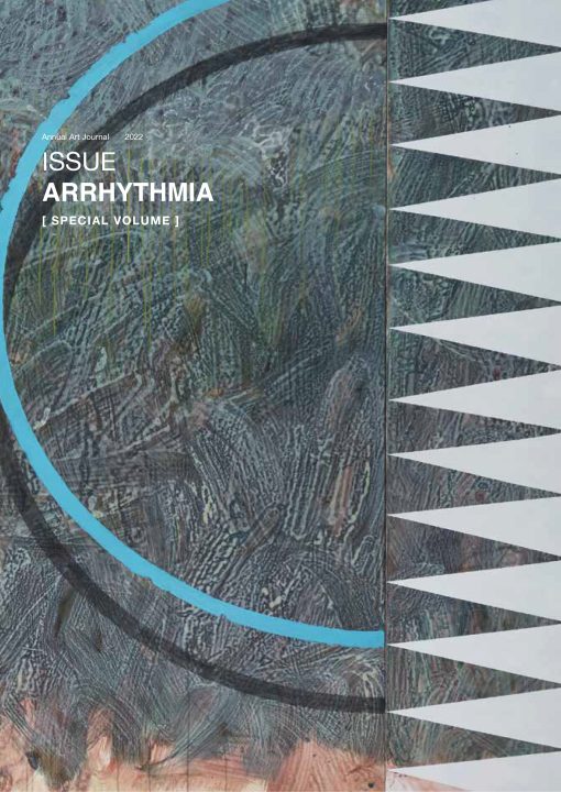
For the purpose of sound modeling, it is helpful to start by thinking of textures as either ‘stationary’ or ‘dynamic.’ Despite their complexity, for some long enough window of time, there is a description of a stationary texture that need not change for different windows of time (figure 1). Sitting next to a babbling brook, we hear the sound as ‘the same’ from minute to minute, even though we know that the sequence of splashes, bubbles, and babbles is never literally the same at two different moments of time. However, if it starts to rain, the brook would change due to the increasing rush and flow. We would describe the sound differently after the rain than before the rain, and this illustrates the dynamic aspect of an audio texture.

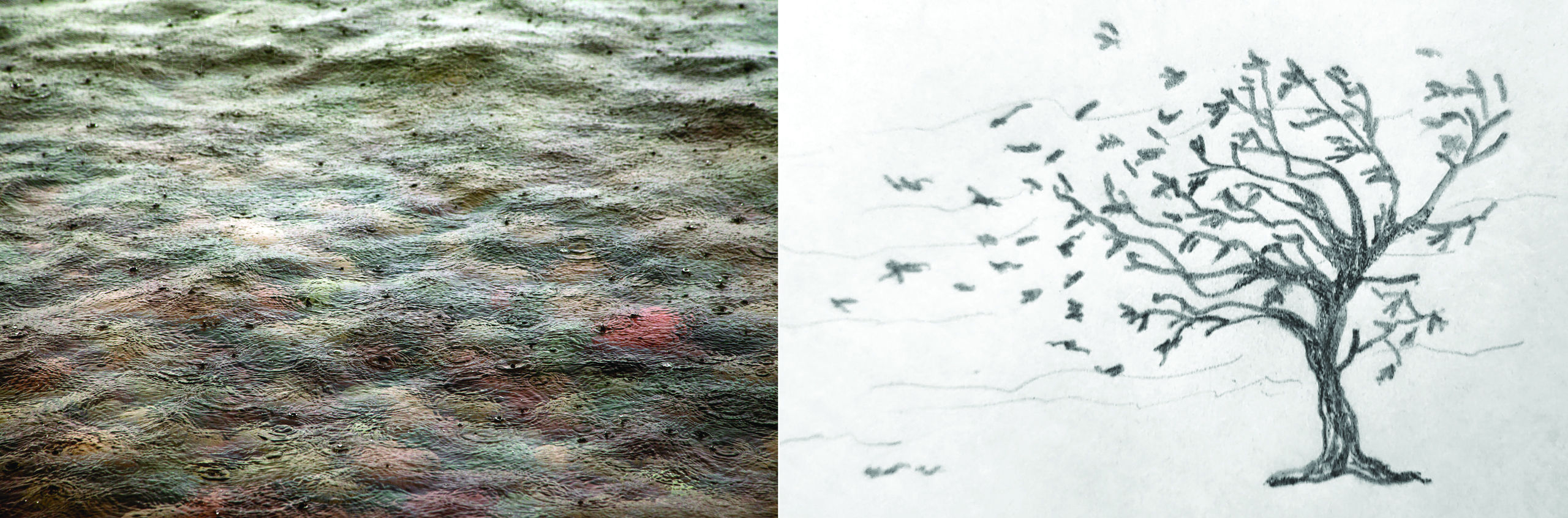
Fig. 1
Left: As long as the rain falls at the same rate, we think of the texture as ‘the same’ even though the sound
(as well as the image on the lake) is never literally identical at different times.
Right: Wind changes at a slower time scale requiring a larger window of time than rain for a ‘stationary’ description.
Image: Lake Superior Rain, Kate Gardiner, CC-NC

 

The distinction between a stationary and dynamic texture is precisely analogous to the distinction between a note and a melody in terms of traditional instruments. The luthier factors out the interactive performative control from the sound generation. The sound of the different static configurations is characteristic of the instrument or model, while the dynamic sequence of configurations defines the imposed expressive or musical content. The sound generation is then conditionally dependent upon the instrument player’s parametric control through an interface.

 

1.3     Previous Texture Modeling Strategies

Computational sound modeling is typically a time and resource-intensive process of writing code. There are a variety of approaches that address the complexity of textures.

One approach is to assemble sounds from a massive set of tiny pieces. Granular synthesis has been theorised and used by multiple musicians: Iannis Xenakis in “Formalized music: thought and mathematics in composition;” Barry Truax in his piece Riverrun and in “Real-time granular synthesis with a digital signal processor” and; Curtis Roads in his “Introduction to granular synthesis” and “Microsound.” The term is used to describe a family of techniques such as assembling windowed sine tones of varying frequencies and windows spanning a few cycles of the wave form. A related technique is called “granulation,” which breaks a recorded sound into tiny pieces before reassembling it.² By specifying various distributions of grains in time, grain signal choices and window sizes, innumerable similar textures can be created. Related techniques include “wavelet analysis and resynthesis”³ and “concatenative synthesis.”⁴

Physical models simulate the actual physical behaviour of sound sources. Simulated plates, tubes, and strings are great for models of pitched instruments, but many physical systems generate more complex textures. For example, the sound of raindrops can be modeled with wave and acoustic pressure equations describing surface impacts.⁵ Other sounds derived from physical phenomena such as bubbling in liquids have been modelled based on fluid simulations).⁶ Rolling, scrapping, and rubbing sounds with a continuous interaction between different objects have been explored.⁷ Perry Cook developed an approach referred to as “physically informed” modeling for sounds such as rattles and footsteps.

 

1.4     A Paradigm Shift

There is a deep interdependence between the sound space that artists work with and the technologies available during the historical time in which they live. The recording technologies (phonographic and magnetic tape) of the early 20th century brought any sound producible in the physical world into the studio and on to the stage. Tape could be speed-controlled and spliced, and vinyl can be scratched, but it was the electronic instruments, and later, digital computers that seemed to promise that any imaginable sound could be synthesised and arbitrarily manipulated performatively. Still, even a synthesiser that can make ‘any sound’ has limits on the ways the sound space can be navigated. The quest continues for the holy grail of access to any and all sound arranged in a designable space for arbitrary navigation. That search is now conducted using the most power-hungry, cloud-based virtually served artificial intelligence machinery. It is driven by artists, engineers, and scientists who might only meet virtually in that same cloud immersed in a communication system that logs their every keystroke as data for AI analysis. Even the pandemic-driven physical isolation seems to drive this mode of production and communication that resonates so deeply with the technologies being developed for artistic exploitation.

Recent years have seen big data and deep learning models disrupt almost every scientific and technical endeavour, and it is no different in the world of sonic arts. Modeling, in particular for generative processes like image and sound synthesis, is now often data driven. Rather than providing a machine with explicitly coded algorithms that execute to produce sound, a learning system is trained to produce media given (usually lots of) data.

Seminal work in data driven modeling of audio textures was done by McDermott and Simoncelli. They studied the human perception of audio textures by generating audio examples to match extracted statistical measurements on noise samples. Their synthesis by analysis approach workswell on sounds with variation at shorter time scales but is less successful on sounds with longer-term structure.⁸ More recently Ulyanov and Lebedev modeled musical textures and others have since applied their approach to general purpose audio.⁹

The next section takes a deeper dive into four specific deep learning architectures that have been effectively used to address the challenge of synthesising complex and noisy data such as natural sound textures.

 

2      A Sound Modeling Toolset

To the uninitiated, the suite of tools in a violin-makers workshop are a large and curious-looking set. From thickness calibrators to router guides, peg hole reamers, gaugers, planers, and purfling tools, the specialised and motley collection bear names as colourful as the tools themselves. So it is for the modern-day sound model designer. In this section we will discuss four important tools hanging on the wall of the sound modelers workshop: The Generative Adversarial Network (GAN), the Self-Organizing Map (SOM), the Style-Transfer Network (STN) and the Recurrent Neural Network (RNN). I will furthermore give these tools more familiar nicknames: the Interpolator, the Smoother, the Variator, and the Performer (figure 2), which better describe their functionality. Like the tools on any workbench, each has its own function and using one to do the job of another can only lead to disaster.

 

2.1    The Interpolator

We have high demands and expectations for data-driven synthesiser design: when we train a system with data, we want a system that can generate not only the sounds in the training data set, but a ‘filled out’ space of sounds. That is, we demand that our system create novel sounds, even if such sounds do not come from the physical world. If we provide sounds of rain and the din of forest bugs as training data, then we expect to play a ‘morph’ on the new instrument in the same way we play a scale between pitches on a violin. The Interpolator (GAN) is a somewhat unwieldy tool for sound design, but it does construct a navigable high-dimensional space where in some regions it generates sounds like those in the data set, and for the rest of the space, it invents convincing ‘in-between’ sounds.

The tool gets its formal name (Generative Adversarial Network) from the way it is structured in two parts. The first part (the Generator) learns to organise a map from an input space of parameters to a set of sounds that are distributed similarly to the dataset. The second part (the Discriminator), is tasked with learning to recognise sounds from the Generator vs. sound from the database (figure 2(a)). The two networks are ‘adversaries’ as the Generator trains to fool the Discriminator. When training completes, and the Discriminator can no longer differentiate between the real and synthetic sounds, we have the Generator we seek.

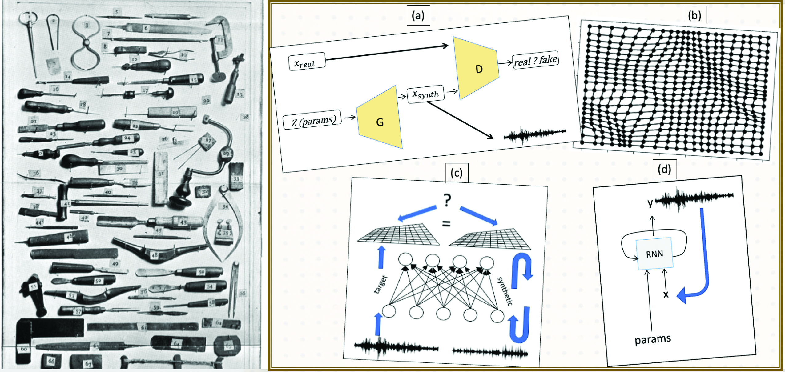
Fig. 2
Left: Violin maker’s toolset.
Right: Sound modeler’s toolset, (a) The Interpolator (GAN) learns to create novel ‘tween’ sounds as the generator G trains
to fool the discriminator D, (b) The Smoother (SOM) makes distances between sounds more uniform as it resamples the
parameter space, (c) The Variator (SNT) creates stationary textural variations by
matching network activation statistics of a
target texture, and (d) The Performer (RNN) generates sound one sample at a time in response to parameters.
Image: Project Gutenberg EBook of Violin Making

 

To appreciate the nature of this tool, the first thing to note is that it creates a map from a large number of input parameters to sound characteristics. This is what is meant by ‘creating a space’ for the sounds, and mapping is done by the tool, not the sound designer. The sound designer must figure out what the parameters actually do to the sound after training! Secondly, the number of input parameters is much larger than those we typically use to control an instrument. The network might require over 100 dimensions in order to organise a sensible space, but for an instrument to be playable by a human, it must offer a far smaller number.

Reflecting on how the Interpolator does its job, provides some insight into the relationship between technology and our historical times. The machine requires a certain amount of autonomy to do its job properly. We can provide some guidance by encoding and communicating our objectives, but we can not micromanage its organisation of the sound space. In fact, to meet our goals for synthesising and interacting with natural and novel sounds, there is generally far too much data address and the synthesis algorithms learned by the machine are too complex for mere mortals to organise or manually design. The process depends on yielding what may have previously been considered creative decision making to the machine.

The self-organisation and generation of novelty only address part of the playability requirements. A limitation of the Interpolator is that it learns long (e.g. 4-second) chunks of sound for each parameter, so is structurally incapable of being ‘played’ in response to continuously varying control parameters. Furthermore, it generates a single sound for each point in the space, not the infinite number of variations we associate with a texture of a given description such as the ever-changing sound of a river with a particular rate of flow. This is a job for the Variator described below.

 

2.2     The Smoother

The Interpolator distributes sound in a parametric space but does not necessarily do so evenly. That is, large parts of the space can be devoted to one or another type of sound and moving over the border from the territory of one to the territory of another might happen very quickly. We want to expand the transitions, and the great thing about the Interpolator’s space is that it can be zoomed infinitely. An analogy to this smoothing process would be zooming in on dusk and dawn so that they last as long as day and night.

The Smoother’s Self Organizing Map (SOM) can learn to create a map of a data distribution with a two-dimensional grid-like representation (figure 2(b)).¹⁰ Playing the remapped instrument, we would move quickly through the regions of sound space where nothing much changes as you navigate, and dwell in the unstable and changing regions between them. To exploit an acoustic instrument analogy again, it would be akin to removing the fret bars from a guitar which cause the pitch to be the same for fingering positions between them so that it would behave more like a (fretless) violin where changes happen smoothly as a finger glides along the neck. This is more natural for textures that do not lend themselves to standardised discrete scales in the way that legacy musical instruments do. It is probably not just an accident of history that we can see the less categorically punctuated and metrical lives we are now living reflected in the borderless sound space of textures that comprise so much sound art today. The Smoother is a tool that literally expands the space and time at narrow border regions turning them into spaces in their own right for the discovery of novel sound that might otherwise go unnoticed.

 

2.3     The Variator

The essence of textures is infinite variation, and for this we reach for another deep learning tool, the Style-transfer networks (STN). Most people have encountered STN’s in the image domain where they take style and textural elements from one image such as a painting to generate a variation on the ‘content’ of another¹¹ (figure 3), thus our nickname, the Variator. It can also be used without content, to simply reproduce images with a similar texture to the original. The network can be used the same way for sound.

Fig. 3 Style transfer networks have been used in the image domain to superimpose the style of one image
(van Gogh’s The Starry Night, inset) onto content from one image (left) to produce new images (right).
Images: Gatys et al. “A neural algorithm of artistic style”

 

The way this tool works is that a segment of sound exhibiting the ‘target’ texture is fed into a neural network. Then the feature activation pattern of one or more network layers are correlated with each other in a time-independent way. Features might represent anything from a short rhythmic pattern, to how pitched an event is. The matrices of feature characteristics are represented by the grids at the top of figure 2(c).

Next, we use the network and the target matrix of feature correlations to construct new sounds. We do that by feeding random noise into the network, deriving its feature characteristics and tweaking the noise until its feature’s characteristics match that of the target. When the process completes, we have a new sound with the texture of the target, but a different temporal structure or variation (figure 4).

This tool has a profoundly beautiful nature: the neural network that serves as the audio feature extractor need not be trained. The same network works as well for sounds of birds flying, rain falling, air conditioners humming, rocks rolling, or cattle bellowing. Indeed, the network need not be trained at all, and features can be entirely random. It seems to matter not what the audio features actually are, but rather what the pattern of relationships between features is.

The Variator also works on an aspect of textures that have a very particular alignment with a common experience of patterns of contemporary life in the time of a pandemic, and that is that it can create an endless series of sounds that, despite their infinite variety, all sound in some way ‘the same.’

In summary, the Variator generates variations of a static texture for a particular instrumental configuration. However, it does not provide the dynamic textures for which playable reconfigurations of instruments are required.

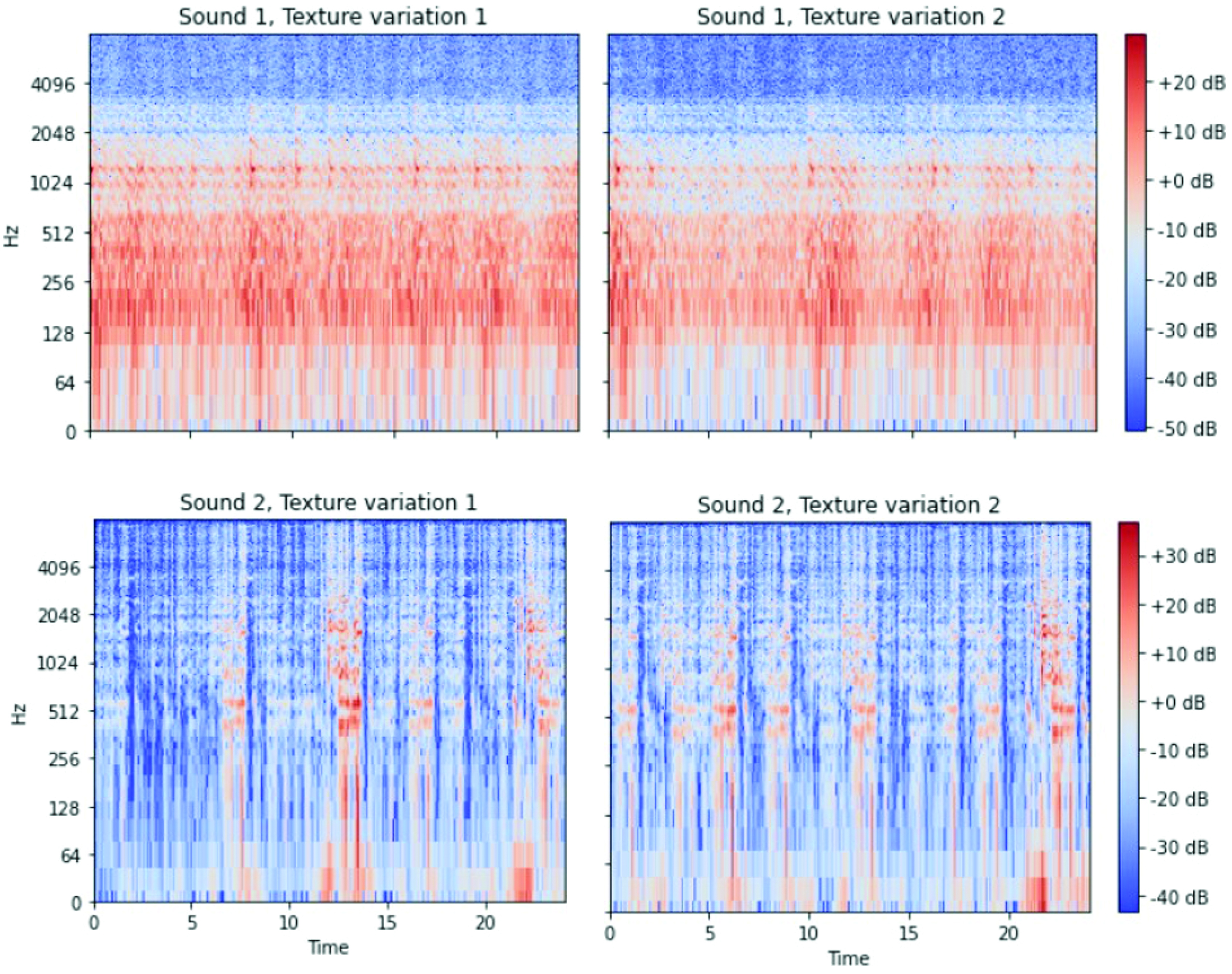
Fig. 4 The two rows correspond to two different dynamic parameter settings.
Each column shows textural variations of the sound for those parameter settings.

2.4    The Performer

The Performer is oriented toward generating sound sequentially in time, unlike the Interpolator and the Variator which generate fixed duration chunks of sound. It gets its formal name, Recurrent Neural Network (RNN), from the fact that the audio output from each step is fed back in as input along with the parameters to create the network state that produces the next sample (figure 2(d)). It provides the playable parametric interface for a musician and generates sound samples that are immediately responsive to parametric input from the instrumentalist one at a time.

When we train the Performer, we provide whatever parameters we want to use to interact with the sound. This network learns to map the parameters and the previous sound sample, together with its current state of activation, to the next sound sample in time. As instrument designers, we choose what the parameters mean by associating them with the specific sequences of sound we want the model to produce. Thus, if we want an interface parameter to control the ‘roughness’ of a scratching sound or the speed of a steam engine, we simply pair appropriate values for the parameter with the sounds we expect them to generate. The Performer learns the mapping.

The mapping from interface to sound need not be deterministic. That is, if we pair a ‘flow rate’ parameter to a rushing water sound, the model can, like the brook it is modeling, generate endless variations of the stationary processes associated with a single input parameter configuration, never repeating the exact same sound sequence. It is at the same time capable of a dynamic range of sounds responding to different configuration parameters—for example for flow rate.

 

3      The Toolset Working as an Ensemble

No craftsperson would use a single tool for all jobs. The tools discussed above all have complementary strengths and weaknesses in the same way that a violin luthier’s router and purfling set do. As an example of texture instrument building, the Interpolator was trained on a set of one-second texture sounds from sound artist Brian O’Reilly, from which we extract a two-dimensional slice for dynamic musical control with two parameters.¹² After the Smoother adjusts the spacing between sounds, the Variator generates extended stationary variations at each parameter point. Finally, the Performer is trained so that the sound can be generated continuously as the space is explored musically by a human performer. A visualisation of how the Interpolator, the Smoother, the Variator and the Performer all work together can be seen in figure 5 and auditioned online at https://animatedsound.com/arrhythmia2021.

 

4      Final Reflections

The noisy and complex sounds that constitute such an important part of contemporary sound art practices are fiendishly difficult to model using traditional approaches to signal processing and computer programming. New deep learning approaches are synergistically evolving, with contemporary artistic interest in exploring the multi-scale complexity of natural sounds that are situated in a world that is itself evermore computationally created, mediated, and richly textured.

The tools described herein are being explored by artists in a variety of media, representing a space of convergence for exploring themes such as creative partnerships with machines, questions of authorship, the incorporation of massive amounts of data in artistic production, and many others. Whether the machines are mobilised for text generation, choreography, visual arts, or music, they generally require a different mode of interaction with artists than traditional tools. Rather than explicit control through physical manipulation or programming, the artist might interact with the more autonomous tools by providing training data or communicating through visual or speech channels. Often the artist evaluates and curates the output from the machines. The style transfer network (Variator) is one such example that emerged first in the visual domain. The artist ‘guides’ its behaviour with target images for content and/or texture, but the machine makes the actual images (or sounds) for the artist.

There are both aesthetic and functional reasons for striking different balances between control and indeterminacy in the tools described here and the creative use of sound they support. No claims about the right way to think about sound art are intended with this approach to sound modeling with its separation of control and texture generation. The practice of modeling and instrument interface design is necessarily explicit about which aspects of a sound are controllable and which are left open to textural variation, but the tool set we have been exploring supports various ways of making choices framing the way we hear, interact with, and make complex sound as part of the design process.

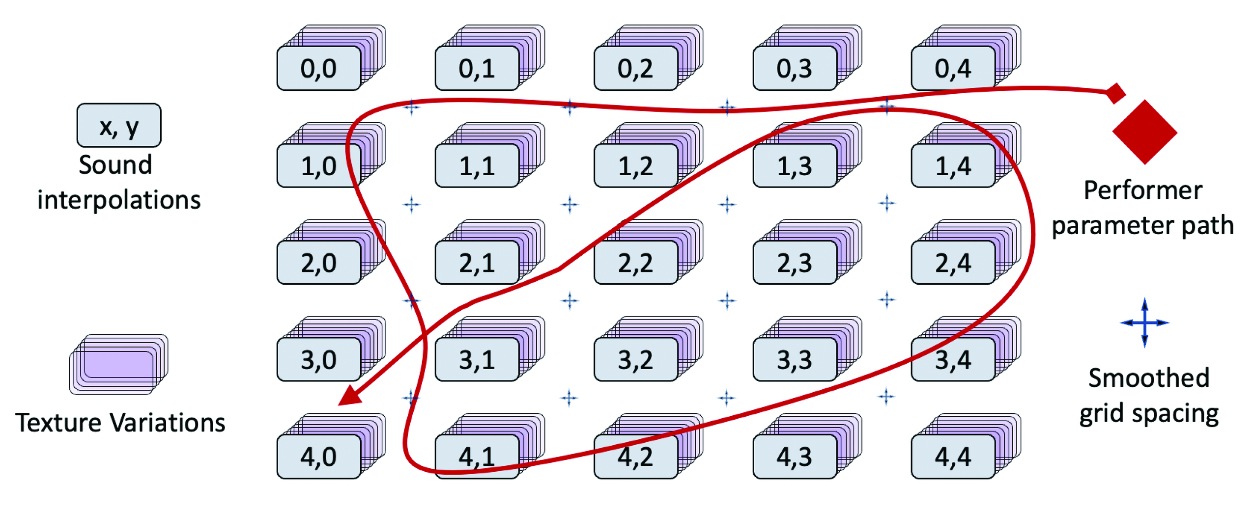
Fig. 5 Each of the four tools presented accomplishes a unique and critical part to the instrument building processes.
The Interpolator fills out a space of dynamic textures (indexed here by parameter pairs x and y), the Smoother adjusts the
space to more evenly spread the interpolations, the Variator creates different stationary textures (shown stacked) at each
point, and the Performer makes the space playable along paths under instrumental control.
(To listen to how these tools work, visit https://animatedsound.com/arrhythmia2021)

 

The focus of this paper has been on modeling audio textures that extend our musical legacy of pitched sounds and regular metres. The data-driven instrumental sound design process also differs from a traditional lutherie in that it reflects a conception of a space of sound that is infinitely generative and configurable rather than one for which there could ever be a definitive set of canonical instruments for playing. While these new sound design processes are inextricably entwined with the very computational and communication technologies that too often oppress, surveil, misinform, and isolate us, they subvert these tendencies with their rich creative musical potential.